Steganography Challenge with Arnold’s Cat Map
Introduction
Today we’ll tackle an intriguing image steganography challenge titled “This is not Arnold’s cat” worth 100 points. This challenge demonstrates how chaotic transformations can be used to hide information in plain sight.
The first step in any steganography challenge is identifying the transformation method applied to the image. In this case, the answer lies within the challenge’s name itself - it references Arnold’s cat map, a fascinating mathematical transformation.
What is Arnold’s Cat Map?
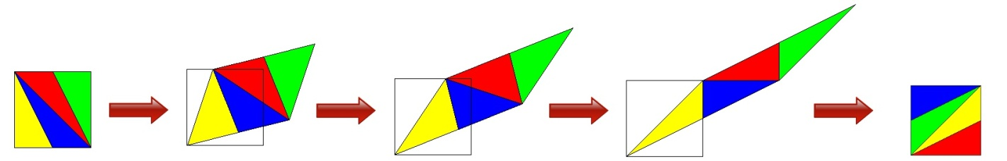
Arnold’s cat transformation (ACT) is a chaotic transformation that systematically shuffles the pixels of an image. Named after the Russian mathematician Vladimir Arnold, who first demonstrated it using an image of a cat, this transformation has the remarkable property of eventually returning to the original image after enough iterations.
The transformation works by applying a specific mathematical formula to each pixel’s coordinates, creating a seemingly random scrambling effect. Despite appearing chaotic, the transformation is completely deterministic and reversible.
The most important thing is that we can retrieve the original image with n iterations. It’s a period.
Understanding the Transformation
While I won’t delve into the complex mathematical details of how ACT works under the hood, what’s crucial for solving this challenge is understanding how the transformation is applied and, more importantly, how to reverse it.
The transformation is defined by the following formula:
\[\begin{pmatrix} x_{n+1} \\ y_{n+1} \end{pmatrix} = \begin{pmatrix} 1 & 1 \\ 1 & 2 \end{pmatrix} \begin{pmatrix} x_n \\ y_n \end{pmatrix} \mod N\]This can also be written in expanded form as:
- $x_{n+1} = (x_n + y_n) \mod N$
- $y_{n+1} = (x_n + 2y_n) \mod N$
Where $(x_n, y_n)$ represents the current pixel coordinates, and $N$ is the image dimension (assuming a square image).
Let’s code
First we need to open our image, of course I will not reveal the flag here so I will use a picture of my cat.
We will use PIL for image management, numpy to manipulate image data and matplotlib to display it.
from PIL import Image
from numpy import asarray
import matplotlib.pyplot as plt
Next, load image :
image = Image.open('vlad.png')
data = asarray(image)
We can now begin implementing ACT. Here is the algorithm:
Algorithm: Arnold’s Cat Map Transformation
ALGORITHM apply_act(data)
    INPUT: data - a square image matrix of size N×N
    OUTPUT: new_data - the transformed image matrix

    N ← dimension of data (assuming square image)
    new_data ← copy of data

    FOR i FROM 0 TO N-1 DO
        FOR j FROM 0 TO N-1 DO

            x ← j
            y ← i

            new_x ← (x + y) MOD N
            new_y ← (x + 2×y) MOD N

            new_data[new_y, new_x] ← data[i, j]
        END FOR
    END FOR

    RETURN new_data
END ALGORITHM
Now here’s the Python implementation:
def apply_act(data):
    N = data.shape[0]
    new_data = data.copy()

    for i in range(data.shape[0]):
        for j in range(data.shape[1]):
            x, y = j, i
            new_x = (x + y) % N
            new_y = (x + 2*y) % N
            new_data[new_y, new_x] = data[i, j]

    return new_data
We define the number of transformation iterations knowing that if $N = 2^n$, then $\text{period} = 3 \times 2^{n-1}$.
For our image vlad.jpg which is 256×256:
We can now apply this transformation for $n = 384$ iterations.
For N = 2^8 = 256, the theoretical upper bound is 384, but empirically the period is 192. Testing up to 384 iterations guarantees finding the original image.
image_grid = [image]

n = 384

for loop in range(n):
    data = apply_act(data)
    new_image = Image.fromarray(data)
    image_grid.append(new_image)
In order to see when original image is retrieve, I create a grid with each iteration transformation.
Finally we can save the grid :
cols = 16
rows = (len(image_grid) + cols - 1) // cols
fig, axes = plt.subplots(rows, cols, figsize=(32, rows*2))

for i, ax in enumerate(axes.flat):
    if i < len(image_grid):
        ax.imshow(image_grid[i], cmap='gray')
        ax.set_title(f'{i}')
    ax.axis('off')

plt.tight_layout()
plt.savefig('grid.png', dpi=150, bbox_inches='tight')
Results
First iterations (0 → 3)
The image quickly becomes unrecognizable as pixels are shuffled according to the transformation matrix:

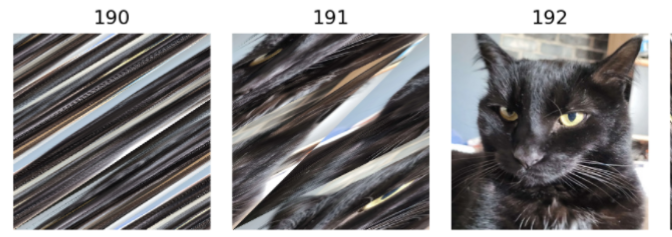
Mid-cycle chaos
At this point, the image appears completely scrambled with no discernible pattern:

Return to original
As we approach iteration 192 (and again at 384), something remarkable happens: the image progressively reconstructs itself and returns to its original state:
This periodic behavior is the key to solving the CTF challenge: by applying enough iterations of Arnold’s Cat Map to a scrambled image, we can recover the hidden flag.